Using Lasagne for training Deep Neural Networks
There are a lot of Deep Learning libraries out there, and the best library really depends on what you are trying to do.
After using the libraries cuda-convnet and Caffe for a while, I found out that I needed more flexibility in the models, in terms of defining the objective functions and in controlling the way samples are selected / augmented during training.
Looking at alternatives, the best options to achieve what I wanted were Torch and Theano. Both libraries are flexible and fast, and I chose Theano because of the language (Python vs Lua). There are several libraries built on top of Theano that make it even easier to specify and train neural networks. One that I found very interesting is Lasagne.
Lasagne is a library built on top of Theano, but it does not hide the Theano symbolic variables, so you can manipulate them very easily to modify the model or the learning procedure in any way you want.
This post is intended for people who are somewhat familiar with training Neural Networks, and would like to know the lasagne library. Below we consider a simple example to get started with Lasagne, with some features I found useful in this library.
CNN training with lasagne
We will train a Convolutional Neural Network (CNN) on the MNIST dataset, and see how easy it is to make changes in the model / training algorithm / loss function using this library. First, install the Lasagne library following these instructions. The actual code to accompany this blog post, as an iPython notebook, can be found here: show me the code!
Now, let’s describe the problem at hand.
The problem
We will consider the MNIST classification problem. This is a dataset of handwritten digits, where the objective is to classify small images (28x28 pixels) as a digit from 0 to 9. The samples on the dataset look like this:
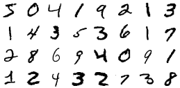 Samples from the MNIST dataset
From a high level, what we want to do if define a model that identifies the digit (\(y \in [0,1,...,9]\)) from an image \(x \in \mathbb{R}^{28*28}\). Our model will have 10 outputs, each representing how confident the model is that the image is a particular number (the probability \(P(y \vert x)\)). We then consider a cost function that considers how wrong our model is, on a set of images - that is, we show a bunch of images, and check if the model is accurate in predicting \(y\). We start our model with random parameters (so in the beginning it will make a lot of mistakes), and we iteratively modify the parameters of the model so that it makes less errors.
The model
Let’s consider a Convolutional Neural Network model proposed by Yann Lecun in the early 90’s. In particular, we will consider a variant of the original architecture called LENET-5 [1]:
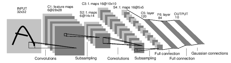 The LENET-5 architecture
Defining the model in lasagne
We will start by defining the model using the Lasagne library. The first step is creating symbolic variables for input of the network (images) and the output - 10 neurons predicting the probability of each digit (0-9) given the image:
1
2
3
4
5
data_size=(None,1,28,28) # Batch size x Img Channels x Height x Width
output_size=10 # We will run the example in mnist - 10 digits

input_var = T.tensor4('input')
target_var = T.ivector('targets')
In this example, we named the inputs as input_var and the outputs as target_var. Notice that these are symbolic variables: they don’t actually contain the values. Instead, they represent these variables in a series of computations (called a computational graph). The idea is that you specify a series of operations, and later you compile a function, so that you can actually pass inputs and receive outputs.
This may be hard to grasp initially, but it is what allows Theano to automatically calculate gradients (derivatives), which is great for trying out new things, and it also enables the library to optimize your code.
Defining the model in Lasagne can be done very easily. The library implements most commonly used layer types, and their declaration is very straightforward:
1
2
3
4
5
6
7
8
9
10
11
12
13
14
15
16
17
18
19
20
net = {}

#Input layer:
net['data'] = lasagne.layers.InputLayer(data_size, input_var=input_var)

#Convolution + Pooling
net['conv1'] = lasagne.layers.Conv2DLayer(net['data'], num_filters=6, filter_size=5)
net['pool1'] = lasagne.layers.Pool2DLayer(net['conv1'], pool_size=2)

net['conv2'] = lasagne.layers.Conv2DLayer(net['pool1'], num_filters=10, filter_size=5)
net['pool2'] = lasagne.layers.Pool2DLayer(net['conv2'], pool_size=2)


#Fully-connected + dropout
net['fc1'] = lasagne.layers.DenseLayer(net['pool2'], num_units=100)
net['drop1'] = lasagne.layers.DropoutLayer(net['fc1'],  p=0.5)

#Output layer:
net['out'] = lasagne.layers.DenseLayer(net['drop1'], num_units=output_size,
                                       nonlinearity=lasagne.nonlinearities.softmax)
Lasagne does not specify a “model” class, so the convention is to create a dictionary that contains all the layers (called net in this example).
The definition of each layer consists of the input for that layer, followed by the parameters for the layer. In line 7 we specify the first layer called conv1. It is a Convolutional Layer that receives input from the layer data, and has 6 filters of size 5x5.
Defining the cost function and the update rule
We now have our model defined. The next step is defining the cost (loss) function, that we want to optimize. For classification problems, the common loss is the cross entropy loss, which is also implemented in lasagne. We will also add some regularization in the form of L2 weight decay.
1
2
3
4
5
6
7
8
9
10
11
12
#Define hyperparameters. These could also be symbolic variables
lr = 1e-2
weight_decay = 1e-5

#Loss function: mean cross-entropy
prediction = lasagne.layers.get_output(net['out'])
loss = lasagne.objectives.categorical_crossentropy(prediction, target_var)
loss = loss.mean()

#Also add weight decay to the cost function
weightsl2 = lasagne.regularization.regularize_network_params(net['out'], lasagne.regularization.l2)
loss += weight_decay * weightsl2
In line 6, we get a symbolic variable of the output layer (which is our prediction \(P(y \vert x)\)). We then obtain the cross entropy loss. Since we will be training with mini-batches, line 7 will return a vector of losses (one for each example). In line 8 we just consider the average of the losses in the mini-batch.
We then add regularization in line 11. It is worth noting how easy it is to add elements to the cost function. Looking at lines 11 and 12, in order to add weight decay we simply need to sum the weight decay to the loss variable.
For training the model, we need to calculate the partial derivatives of the loss with respect to the weights in our model. Here is where Theano really shines: since we defined the computations using symbolic math, it can automatically calculate the derivatives of an arbitrary loss function with respect to the weights.
Lastly, we need to select an optimization procedure, that defines how we will update the parameters of the model.
1
2
3
4
#Get the update rule for Stochastic Gradient Descent with Nesterov Momentum
params = lasagne.layers.get_all_params(net['out'], trainable=True)
updates = lasagne.updates.sgd(
        loss, params, learning_rate=lr)
Here we used standard Stochastic Gradient Descent (SGD), which is a very straightforward procedure, but we can also use more advanced methods, such as Nesterov Momentum and ADAM very easily (see the code for examples). Note that the classes in lasagne.updates also encapsulate the call to Theano to obtain the gradients (the partial derivatives of the loss with respect to the parameters).
Compiling the training and testing functions
We now have all the variables that define our model and how to train it, the next step if to actually compile the functions that we can run to perform training and testing.
1
2
3
4
5
6
7
8
9
10
11
train_fn = theano.function([input_var, target_var], loss, updates=updates)

test_prediction = lasagne.layers.get_output(net['out'], deterministic=True)
test_loss = lasagne.objectives.categorical_crossentropy(test_prediction,
                                                        target_var)
test_loss = test_loss.mean()
test_acc = T.mean(T.eq(T.argmax(test_prediction, axis=1), target_var),
                  dtype=theano.config.floatX)

val_fn = theano.function([input_var, target_var], [test_loss, test_acc])
get_preds = theano.function([input_var], test_prediction)
The first line compiles the training function train_fn, which has an “updates” rule. Whenever we call this function, it updates the parameters of the model.
\(\DeclareMathOperator*{\argmax}{arg\,max}\) We have defined two functions for test: the first is val_fn, that returns the average loss and classification accuracy of a set of images and labels \((x,y)\), and get_preds, that returns the predictions \(P(y \vert x)\), given a set of images \(x\). The accuracy is calculated as follows: we consider that the model predicts the class \(y\) that has the largest value of \(P(y \vert x)\) for a given image \(x\). That is \(\hat{y} = \argmax_y{P(y \vert x)}\). We compare this prediction with the ground truth, and take the average value over the entire test set.
Training the model
To train the model, we need to call the training function train_fn for mini-batches of the training set, until a stopping criterion.
1
2
3
4
5
6
7
8
9
10
#Run the training function per mini-batches.
n_examples = x_train.shape[0]
n_batches = n_examples / batch_size

for epoch in xrange(epochs):
    for batch in xrange(n_batches):
        x_batch = x_train[batch*batch_size: (batch+1) * batch_size]
        y_batch = y_train[batch*batch_size: (batch+1) * batch_size]

        train_fn(x_batch, y_batch) # This is where the model gets updated
Here we simply run the model for a fixed number of epochs (iterations over the entire training set). In each epoch, we use mini-batches: a small set of examples that is used to calculate the derivatives of the loss with respect to the weights, and update the model. Since our training function returns the loss of the mini-batch, we could also track it to monitor progress (this is done in the code).
Running this code on a Tesla C2050 GPU takes around 10 seconds per epoch. I ran it for 50 epochs for a total of 490 seconds (a little over 8 minutes).
Testing the model
Now that the model is trained, it is very easy to get predictions on the test set. Let’s now get the accuracy on the testing set:
loss, acc = val_fn(x_test, y_test)
test_error = 1 - acc
print('Test error: %f' % test_error)
With the model trained for 50 epochs, the test error we achieve is \(0.8\%\). All 10000 test images are classified in 0.52 seconds.
And that is it. We have defined our model, trained it for a fixed number of epochs on the training set, and evaluated its performance on a testing set.
Here are some predictions made by this model:
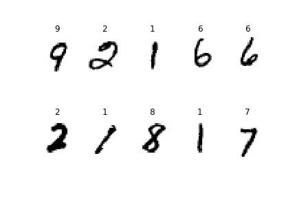 Predictions of random images from the testing set
The model seems to be doing a pretty good job. Let’s now take a look on some cases where the model failed to predict the correct class:
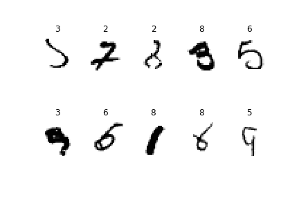 Incorrect predictions in the testing set
There is certainly room for improvement in the model, but it is entertaining to see that the cases that the model gets wrong are mostly hard to recognize.
Making changes
The nice thing about this library is that it is very easy to try out different things. For instance, it is easy to change the model architecture, by adding / removing layers, and changing their parameters. Other libraries (such as cuda-convnet) require that you specify the parameters in a file, which is harder to use if you want to, for instance, try out different numbers of neurons in a given layer (in an automated way).
Another thing that is easy to do in lasagne is using more advanced optimization algorithms. In the code I added an ipython notebook that trains the same network architecture using Stochastic Gradient Descent (SGD) and some more advanced techniques: RMSProp and ADAM. Here is a plot of the progress of the training error over time (in epochs - the number of passes through the training set):
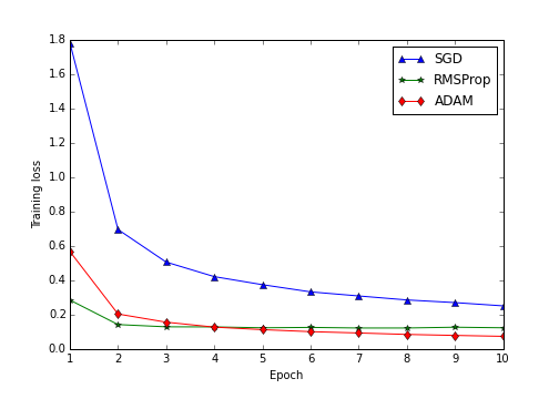 Training progress with different optimization algorithms
For this dataset and model, using ADAM was much superior than the classical Stochastic Gradient Descent - for instance, in the second pass on the training set (using ADAM), the performance was the same as doing 10 epochs using SGD. Testing out different optimization algorithms is very easy in Lasagne - changing a single line of code.
Other things you can easily do:
- Add terms to the cost function. Just add something to the "loss" variable that is used for defining the updates. Theano will take care of calculating the derivatives with respect to the inputs. For instance, you may want to penalize the weights on a given layer more than the others, or you may want to jointly optimize another criterion, etc.
- It is very easy to obtain the representations on an intermediate layer (which can be used for Transfer Learning, for instance)
output_at_layer_fc1 = lasagne.layers.get_output(net['fc1']) get_representation = theano.function([input_var], output_at_layer_fc1) - You can fine-tuned pre-trained models. By default, the weights are initialized at random (in a good way, following [2]), but you can also initialize the layers with pre-trained weights:
net['conv1'] = lasagne.layers.Conv2DLayer(data, num_filters=32, filter_size=5,
                                   W=pretrainedW, b=pretrainedB)
There are some pre-trained models in ImageNet and other datasets in the Model Zoo.
References
[1] LeCun, Y., Boser, B., Denker, J. S., Henderson, D., Howard, R. E., Hubbard, W., & Jackel, L. D. (1989). Backpropagation applied to handwritten zip code recognition. Neural computation, 1(4), 541-551.
[2] Glorot, X., & Bengio, Y. (2010). Understanding the difficulty of training deep feedforward neural networks. In International conference on artificial intelligence and statistics (pp. 249-256).